Flash ADC priority encoder vhdl design

The priority encoder is useful in many application not only in digital circuit but also in the mixed circuit such as analog to digital converter(ADC). For example Flash type ADC uses priority encoder to select which of the different inputs should be sampled and encoded into digital digital bits. The following shows how Flash type ADC works first then VHDL model for the priority encoder is developed.

There are different types of ADC and one of them is Parallel Comparator ADC or Flash ADC. The Flash ADC converts analog signal to digital signal very fast compared to other types of ADC such as Dual Slope ADC or Successive Approximation Register(SAR) ADC. That is its conversion time is small. The disadvantage of Flash ADC is that if the resolution is to be increased then the number of comparator has to be increased which makes the converter bulky.

The Flash ADC can be described as being composed of 3 different constituents- the Voltage Divider Resistor(VDR) network, the Comparators(op-amp) and the priority encoder.

The VDR network is used to create voltage reference with which the input analog signal is compared using the comparator. The voltage reference points is created using same value resistor and the number of the reference points to be created is decided by the number of digital bits one wants to produce. As an example, if n=3 bits is used for the digital signal output then the number of the voltage reference point is 2^3-1= 7. Next the input analog signal which is to be converted into digital signal is done by fedding the analog signal to the inputs of the comparators. The analog signal is fed into the non-inverting terminal of the op-amp and the voltage references are connected to the inverting terminal of the op-amp. The output of those op-amp becomes high in which the input signal voltage is greater than the reference voltage. If there are 7 op-amps comparator, then the analog signal voltage becomes greater than the reference voltage starting from the 3rd op-amp then the rest of the op-amp output also becomes high. That is the 3rd, 4th, 5th, 6th and 7th op-amp output are high.

The priority encoder gives priority to that op-amp output which is first activated high, in this case the 3rd op-amp. Then the priority encoder outputs digital bits corresponding to the digit 5.

Thus one use of priority encoder is in the ADC converter. Now the following describes how a priority encoder is modelled in VHDL.



The input to the priority encoder for the 3 bits digital signal output from the ADC are the 7 outputs from the comparator(op-amps). Depending upon which output gets activated first we produce corresponding digital outputs.

Let Cinp be the input to the priority encoder and Dcode be the digital codes. Then the entity declaration of this priority encoder becomes-

entity priority_encoder is
    port(
    Cinp : in std_logic_vector(7 downto 0);
    Dcode : out std_logic_vector(2 downto 0)
    );
end priority_encoder;

Next we need to create the architecture for the priority encoder. The following is the VHDL code for the flash type ADC priority encoder:

architecture priority_encoder_arch of priority_encoder is
begin
Dcode <= "111" when (Cinp(7)=1) else
"110" when (Cinp(6)=1) else
"101" when (Cinp(5)=1) else
"100" when (Cinp(4)=1) else
"011" when (Cinp(3)=1) else
"010" when (Cinp(2)=1) else
"001" when (Cinp(1)=1) else
"000"; 
end priority_encoder_arch;

Read More..

Linear Block encoding explanation via Block Diagram

The process of Linear Block encoding and decoding is presented in block diagram form to show the process involved in encoding and decoding.

Linear block code encoder accepts k bits of data blocks and encodes them into n bits of block called codes. The rate of transmission is R = k/n. It is the most simplest form of channel encoding.

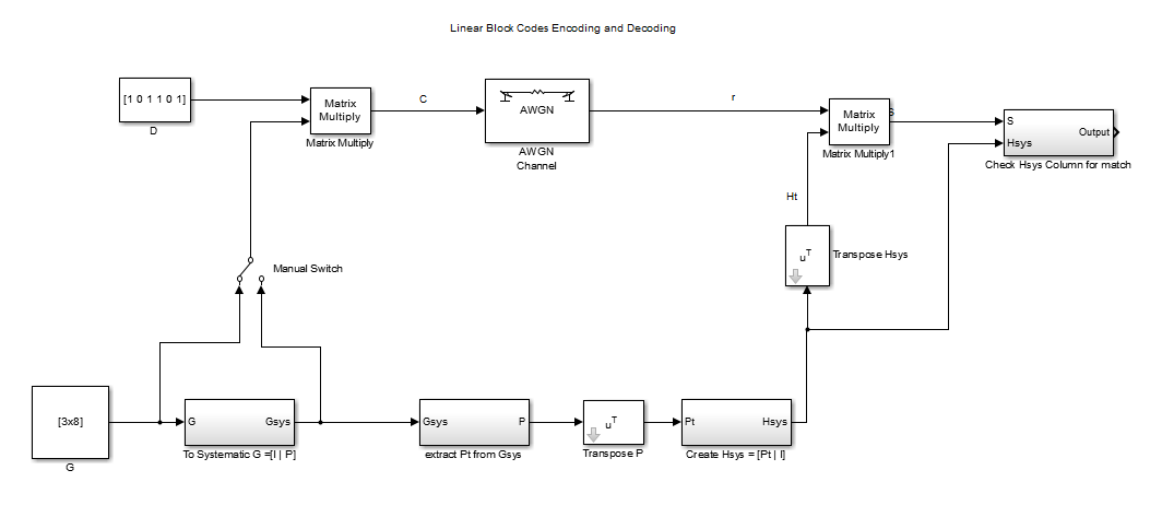
The block diagram below illustrates how the channel encoding in the transmitter side and decoding at the receiving side are performed.

At the transmitter encoder, Data to be encoded is multiplied by the Generator Matrix G. The generator matrix may or may not be in systematic form. A Generator Matrix not in systematic form can always be manipulated via appropriate row operation to get systematic form of the matrix. The switch shows that either the non-systematic form of systematic form of G can be multiplied with the data sequence D to get the code words C.

Now the code words C have been generated and the data is protected. These codewords are entered to the communication channel like the AWGN channel. This block has been shown to illustrate that there is a channel that might corrupt the codewords. After passing through the channel we get received code words r.
r = c+e
where, e is the possible error introduced by the channel.

This received signal r is multiplied by the transposed parity check matrix Ht. t means transposed. Ht matrix is created from the generator matrix. The various steps to get Ht from G or the Gsys(depending upon initial G assumption) is also shown in the block diagram.

If G is not in the systematic form, then it is converted to systematic form Gsys via row operation. Then from Gsys knowledge we can know the Parity sub matrix P. We transpose P to get its transposed form Pt. Then from the knowledge of Pt we can get the H matrix and by taking the transpose of H we get Ht.

This Ht is now multiplied by the received code vector r get the Syndrome vector S. S is then analyzed to get information about error and correct error if possible. First if S is zero then there is no error and we can strip off the parity bits to get the message data D. Second if S is non-zero than it indicates that there is error. S vector sequence is compared with the column of Hsys to see if there is any match. If there is match in the jth column for example then the jth bit of S is in error and this is then corrected. Then the parity bits are stripped off from the received vector r to get the message data back.

Read More..

Sampling process illustration in Matlab

Here a simple example of sampling process of a signal in matlab is provided. Sampling is effectively applying pulse signal to a transistor that turns it on and off. In matlab this can be stimuated by applying a pulses to an input signal.

Here first impulse(h) is generated using filter and then applied to a sinuoid signal(x) to get the sampled signal(y).

The following line generates an impulse response h.

% generate discrete time impulse signal

a = [1 0 0 0 -1];

d = [1 zeros(1,127)];

h = filter(1,a,d);

n = 0:127;

The following line generates a cosine signal

% generate cosine signal

x = cos(2*pi*n/32);

% generate frequency response for signal x

[X,w] = freqz(x,1,128,whole);

% scale w for plotting properly

wp = fftshift(w)/pi-1;

The frequency spectrum of cosine signal is plotted below,

% plot frequency response of x

figure(1)

plot(wp,X)

Now the cosine signal x is multiplied by h which is effectively the process of sampling.

% sampling with 8 samples/ cycle

y = x.*h;

This sampled signal y is then plotted to get its frequency spectrum

Y = fft(y);

figure(2)

plot(wp,Y);

The overall process is shown in the graph which shows signals and its spectrum at various stages:

The overall matlab code is below,

% generate discrte time impulse signal

a = [1 0 0 0 -1];

d = [1 zeros(1,127)];

h = filter(1,a,d);

n = 0:127;

H = fft(h);

% generate cosine signal

x = cos(2*pi*n/32);

% generate frequency response for signal x

[X,w] = freqz(x,1,128,whole);

% scale w for plotting properly

wp = fftshift(w)/pi-1;

% sampling with 8 samples/ cycle

y = x.*h;

Y = fft(y);

figure

subplot(3,2,1)

plot(n,h)

title(Time Domain Responses)

xlabel(Time)

ylabel(h)

subplot(3,2,2)

plot(n,H);

title(Frequency Responses)

xlabel(Frequency)

ylabel(H)

subplot(3,2,3)

plot(n,x)

xlabel(Time)

ylabel(x)

subplot(3,2,4)

plot(wp,X);

xlabel(Frequency)

ylabel(X)

subplot(3,2,5)

plot(n,y)

xlabel(Time)

ylabel(y)

subplot(3,2,6)

plot(wp,Y);

xlabel(Frequency)

ylabel(Y)

Read More..

How to design a code converter using VHDL

Code converter finds application in digital system design and in this blog it is shown how to design a code converter using VHDL. There are many instances that requires code conversion for example in communication system encoding. For example binary to excess 3 code or binary to gray code or gray code to excess 3 code.

The conversion of codes from one to another can be done in different ways. One way is to construct state diagram. Another way is simply to use case statements or if-then-elsif or select statements. There may be also other ways.

Here it is shown how case statement and select statement can be using to convert binary code to excess 3 code.

The first thing to know is what and how they need to converted. 4bit excess 3 code is obtained by adding 0011 to the 4 bit binary value.

It is helpful to construct a truth table for the conversion.

There are 16 codes listed above, but here only 8 codes will be illustrated as this is enough to illustrate how to implement the conversion.

Let x and y be the input and output respectively, that is x is the binary 4 bit input and y is the 4 bit excess 3 code output.

So the entity declaration would look this,

entity code_converter is
    port(
    x : in std_logic_vector(3 downto 0);
    y : out std_logic_vector(3 downto 0)
    )
end code_converter;

Now to the question of How to design a code converter using VHDL?

First it is shown how select statement can be used to do the code conversion. The architecture for the code converter using the select statment is as follows,

architecture Select_RTL of code_converter is

begin
        with x select
        y <= "0011" when "0000",
        "0100" when "0001",
        "0101" when "0010",
        "0110" when "0011",
        "0111" when "0100",
        "1000" when "0101",
        "1001" when "0110",
        "1010"    when "0111",
        "XXXX" when others;
               
end Select_RTL;

Now the same code conversion can be achieved using case statement as follows,

architecture Case_RTL of code_converter is

begin
    process (x)
    begin
        case x is
            when "0000" => y <= "0011";
            when "0001"    => y <= "0100";
            when "0010"    => y <= "0101";
            when "0011" => y <= "0110";
            when "0100" => y <= "0111";
            when "0101" => y <= "1000";
            when "0110" => y <= "1001";
            when "0111" => y <= "1010";
            when others => y <= "XXXX";
        end case;
       
    end process;
end Case_RTL;

Yet there is another method that can be used to implement this conversion. It is much simpler than the above two methods.

architecture add_RTL of code_converter is

signal y_int : integer;

begin
    y_int <= to_integer(unsigned(x)) + 3;
    y <= std_logic_vector(to_unsigned(y_int,4));

end add_RTL;

In this method, the input binary x was converted to integer and 3 was added to it. The result was converted back to binary bits.

See the tutorial- http://appliedelectronicsengineering.blogspot.com/2014/10/how-to-convert-stdlogicvector-to.html to see how to convert between different data types.

So in this way we can use different methods to design a code converted using VHDL.

Read More..

Approaches to analyze experimentally collected data in Matlab

If you were to analyze two or more random set of data whose dependencies you dont know, how would you proceed to find the relationship of the random variables? In Matab there are many build in function and GUI tools to do this. One is to calculate statistics of which correlation, covariances are important and there is curve fitting with/or regression.

Typical when you have sets of random data, you would see the closeness of the data distribution which is done through correlation(covariance) and/or cross-correlation. The when you see any relation between any two data sets you would proceed to curve fitting.

One way to find the relationship is to find correlation between the data sets. The data set could be linearly or non-linearly relationship. Another similar statistical parameter is the covariance gives the strength of the correlation between the data sets.

This statistics can be calculated in matlab using the following 3 functions-
1. corrcoef
2. cov
3. xcorr

The first corrcoef calculates the correlation coefficient, the second cov function calculates the covariance and the third function xcorr calculates cross-correlation.

Another method of statistical analysis of random data is curve fitting. In this method, a polynomial relates input and output variables via polynomial coefficient.

A generalized polynomial equation is as follows,

y = a1 x^n + a2 x^n-1 +a3 x^n-2 + ......

The Curve fitting problem can be attacked in matlab in two ways. The first is through programming using build in functions polyfit and polyvar and others. The second approach is to use the build in Curve Fittting GUI tool.

Curve Fitting using Programming approach:

There are two matlab function which is used to analyze such polynomial equation- polyfit and polyval.

polyfit calculates the coefficients like a1, a2 .. in the above equation from data x and y. And, polyval calculates y from coefficients and x.

Curve Fitting GUI tool:

Yet another way of analyzing your data is the interactive fitting using the matlab basic fitting tool. Lets illustrate an example on how to use the basic fitting tool in matlab.

Let say you have done some experiment and collected some random data.

To opent the basic fitting tool you need to open the plot window by typing

>> plot(data)

in the matlab command prompt, where data is your random data.

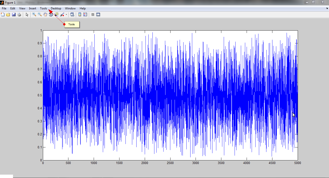
Here is an example of such a plot of random data. Your plot will be different than this.

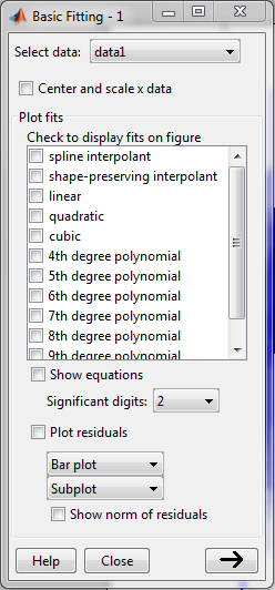
The basic fitting tool is in the Tools>Basic Fitting in the toolbar.

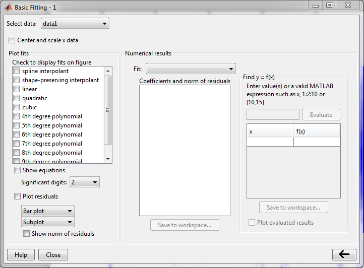
When you click the -> arrow in the above figure then you will get the complete window as shown below,

This tool window basically allows you to

• Select various interpolation algorithms- spline interpolant and polynomial interpolant
• Plot data in various forms
• Compute equation
• compute coefficients, residuals
• export the data

and others

The basic procedure here is now to select the interpolation algorithm that you would like to work with such as cubic or spline. Then you select the sub-option for those algorithms. Then the matlab program tries to fit the data that you have provided.

Read More..

Tutorial For Model Style Effect

Model Style Effect

Material:-
Glitter Stars
Texture
Open the PS
Click On The Photo To Edit
Filter>Noise Reduction>Middle
Filter> Effect Film> Cinema>Middle
Auto Level - Middle
Brightness, Color>Brighten> [2 times]
Open the texture and leave the opacity at 64
& Adjust It On Girl Image
 Click Photo+Objects
Now Open The Stars & adjust Them On Right Side
Click Photo+ObjectsSharpen> 2

Click HOME>Grayscale(If U Use Colour Photo)
Result:-

Read More..

Microstrip Antenna Design Handbook by Ramesh Garg

 Microstrip antenna is becoming essential part of electronics devices. Microstrip antenna are nowadays used in every electronics products due to simplicity of incorporating them into the electronics PCB. The Microstrip Antenna Design Handbook by Ramesh Garg explains the design, model design, analysis, simulation and fabrication of such antenna. Download the pdf ebook from the link below-

http://www.filefactory.com/file/cct1tqlodf9/bhartia.pdf

What are contained within the book?

The book is essentially meant for antenna designers, engineers and scientists. It explains questions like what are the advantages of Microstrip antenna and what are the limitation of Microstrip antenna? What are the various types of antenna? such as Patch antenna, printed dipole antenna, slot antenna and others. What are the feeding techniques, coaxial feeds, coplanar feeds, aperture coupled feed etc.
It also explaines the integration of microstrip antenna with electronics circuits. Antenna array design is also discussed.

Another antenna design book is the Microstrip Patch Antenna: A Designer Guide

See tutorials on design of Microstrip Patch Antenna

Read More..