Tata Sky to invest Rs 900 crore in FY14 eyes 30 growth

Direct-to-home television operator Tata Sky plans to invest Rs 900 crore this fiscal on upgrading technology as it targets a 30 per cent growth in subscribers.

"We will invest around Rs 900 crore to shift to new technology that will help us expand our channel offerings," Tata Sky CEO Harit Nagpal told PTI.

The company will switch to the MPEG-4 format from the current MPEG-2 standard, enabling it to offer more than 300 channels from about 230 now. The changeover is part of Tata Skys strategy to increase its subscriber base, which stands at 10 million.

"We have already started the process of moving over to the new technology. This is likely to be completed by July 2014. We have to change set-top boxes of each of our customers, hence it will take so long," Nagpal said.

Tata Sky is one of six private DTH companies offering services to 56.5 million subscribers as of March 31, according to the Telecom Regulatory Authority of India (TRAI).

"We will grow by 25-30 per cent this financial year," Nagpal said, adding that digitisation has helped to win over former analog cable customers.

DTH companies are adding 8-10 million customers every year as analog cable systems are digitised to allow all TV signals to be provided only through set-top boxes, he said.

The second phase of digitisation of cable TV systems ended on March 31 and covered 38 cities with a population of more than 1 million, according to TRAI. The whole country is expected to be covered by the end of 2014.

Read More..

Sampling process illustration in Matlab

Here a simple example of sampling process of a signal in matlab is provided. Sampling is effectively applying pulse signal to a transistor that turns it on and off. In matlab this can be stimuated by applying a pulses to an input signal.

Here first impulse(h) is generated using filter and then applied to a sinuoid signal(x) to get the sampled signal(y).

The following line generates an impulse response h.

% generate discrete time impulse signal

a = [1 0 0 0 -1];

d = [1 zeros(1,127)];

h = filter(1,a,d);

n = 0:127;

The following line generates a cosine signal

% generate cosine signal

x = cos(2*pi*n/32);

% generate frequency response for signal x

[X,w] = freqz(x,1,128,whole);

% scale w for plotting properly

wp = fftshift(w)/pi-1;

The frequency spectrum of cosine signal is plotted below,

% plot frequency response of x

figure(1)

plot(wp,X)

Now the cosine signal x is multiplied by h which is effectively the process of sampling.

% sampling with 8 samples/ cycle

y = x.*h;

This sampled signal y is then plotted to get its frequency spectrum

Y = fft(y);

figure(2)

plot(wp,Y);

The overall process is shown in the graph which shows signals and its spectrum at various stages:

The overall matlab code is below,

% generate discrte time impulse signal

a = [1 0 0 0 -1];

d = [1 zeros(1,127)];

h = filter(1,a,d);

n = 0:127;

H = fft(h);

% generate cosine signal

x = cos(2*pi*n/32);

% generate frequency response for signal x

[X,w] = freqz(x,1,128,whole);

% scale w for plotting properly

wp = fftshift(w)/pi-1;

% sampling with 8 samples/ cycle

y = x.*h;

Y = fft(y);

figure

subplot(3,2,1)

plot(n,h)

title(Time Domain Responses)

xlabel(Time)

ylabel(h)

subplot(3,2,2)

plot(n,H);

title(Frequency Responses)

xlabel(Frequency)

ylabel(H)

subplot(3,2,3)

plot(n,x)

xlabel(Time)

ylabel(x)

subplot(3,2,4)

plot(wp,X);

xlabel(Frequency)

ylabel(X)

subplot(3,2,5)

plot(n,y)

xlabel(Time)

ylabel(y)

subplot(3,2,6)

plot(wp,Y);

xlabel(Frequency)

ylabel(Y)

Read More..

Approaches to analyze experimentally collected data in Matlab

If you were to analyze two or more random set of data whose dependencies you dont know, how would you proceed to find the relationship of the random variables? In Matab there are many build in function and GUI tools to do this. One is to calculate statistics of which correlation, covariances are important and there is curve fitting with/or regression.

Typical when you have sets of random data, you would see the closeness of the data distribution which is done through correlation(covariance) and/or cross-correlation. The when you see any relation between any two data sets you would proceed to curve fitting.

One way to find the relationship is to find correlation between the data sets. The data set could be linearly or non-linearly relationship. Another similar statistical parameter is the covariance gives the strength of the correlation between the data sets.

This statistics can be calculated in matlab using the following 3 functions-
1. corrcoef
2. cov
3. xcorr

The first corrcoef calculates the correlation coefficient, the second cov function calculates the covariance and the third function xcorr calculates cross-correlation.

Another method of statistical analysis of random data is curve fitting. In this method, a polynomial relates input and output variables via polynomial coefficient.

A generalized polynomial equation is as follows,

y = a1 x^n + a2 x^n-1 +a3 x^n-2 + ......

The Curve fitting problem can be attacked in matlab in two ways. The first is through programming using build in functions polyfit and polyvar and others. The second approach is to use the build in Curve Fittting GUI tool.

Curve Fitting using Programming approach:

There are two matlab function which is used to analyze such polynomial equation- polyfit and polyval.

polyfit calculates the coefficients like a1, a2 .. in the above equation from data x and y. And, polyval calculates y from coefficients and x.

Curve Fitting GUI tool:

Yet another way of analyzing your data is the interactive fitting using the matlab basic fitting tool. Lets illustrate an example on how to use the basic fitting tool in matlab.

Let say you have done some experiment and collected some random data.

To opent the basic fitting tool you need to open the plot window by typing

>> plot(data)

in the matlab command prompt, where data is your random data.

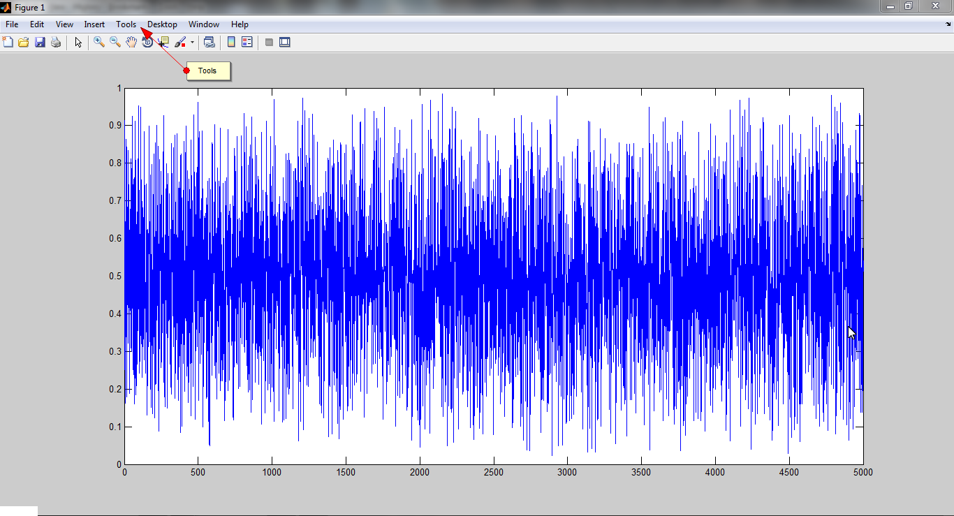
Here is an example of such a plot of random data. Your plot will be different than this.

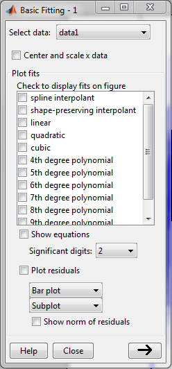
The basic fitting tool is in the Tools>Basic Fitting in the toolbar.

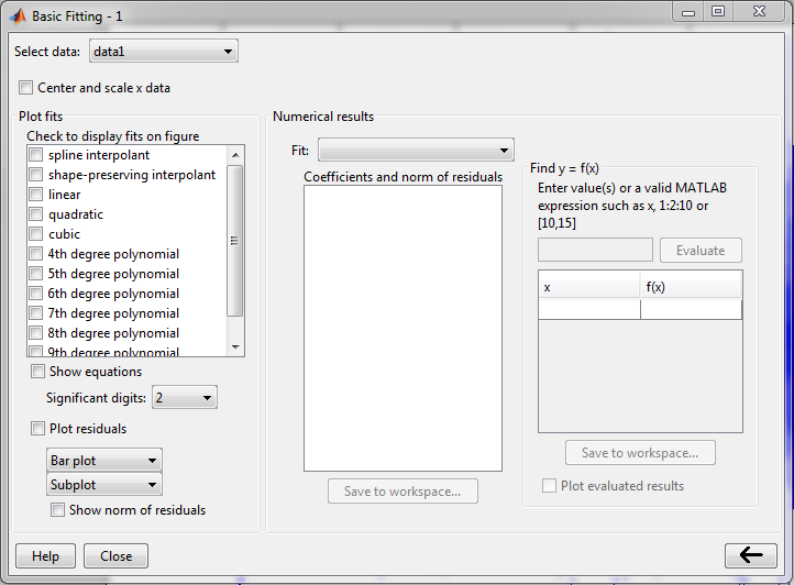
When you click the -> arrow in the above figure then you will get the complete window as shown below,

This tool window basically allows you to

• Select various interpolation algorithms- spline interpolant and polynomial interpolant
• Plot data in various forms
• Compute equation
• compute coefficients, residuals
• export the data

and others

The basic procedure here is now to select the interpolation algorithm that you would like to work with such as cubic or spline. Then you select the sub-option for those algorithms. Then the matlab program tries to fit the data that you have provided.

Read More..

Microsoft Mathematics Add in 2013 for Word and OneNote Available for Download

Free PROGRAMS
Microsoft Mathematics Add-in 2013 for Word and OneNote is now available for download. This add-in makes it easy to plot graphs in 2D and 3D, solve equations or inequalities, and simplify algebraic expressions in your Word documents and OneNote notebooks.

With the Microsoft Mathematics Add-in 2013 for Word and OneNote, you can perform mathematical calculations and plot graphs in your Word documents and OneNote notebooks. The add-in also provides an extensive collection of mathematical symbols and structures to display clearly formatted mathematical expressions. You can also quickly insert commonly used expressions and math structures by using the Equation gallery.

The Microsoft Mathematics Add-in helps you:

Compute standard mathematical functions, such as roots and logarithms.
Compute trigonometric functions, such as sine and cosine.
Find derivatives and integrals, limits, and sums and products of series.
Perform matrix operations, such as inverses, addition, and multiplication.
Perform operations on complex numbers.
Plot 2-D graphs in Cartesian and polar coordinates.
Plot 3-D graphs in Cartesian, cylindrical, and spherical coordinates.
Solve equations and inequalities.
Calculate statistical functions, such as mode and variance, on lists of numbers.
Factor polynomials or integers.
Simplify or expand algebraic expressions.
Download Microsoft Mathematics Add-in 2013 for Word and OneNote
Microsoft Mathematics Add-in 2013 for Word and OneNote is available at the following website.

Microsoft Mathematics Add-in 2013 for Word and OneNote
System requirements
Supported operating systems: Windows 7, Windows 8, Windows Server 2008 R2, Windows Server 2012

Microsoft .NET Framework 4.0
This download works with the following Office programs:
Microsoft Word 2013 and Microsoft OneNote 2013
Microsoft Word 2010 and Microsoft OneNote 2010
Microsoft Office Word 2007
Reference:
Microsoft

program4secure.blogspot.com

Read More..