If you were to analyze two or more random set of data whose dependencies you dont know, how would you proceed to find the relationship of the random variables? In Matab there are many build in function and GUI tools to do this. One is to calculate statistics of which correlation, covariances are important and there is curve fitting with/or regression.
Typical when you have sets of random data, you would see the closeness of the data distribution which is done through correlation(covariance) and/or cross-correlation. The when you see any relation between any two data sets you would proceed to curve fitting.
One way to find the relationship is to find correlation between the data sets. The data set could be linearly or non-linearly relationship. Another similar statistical parameter is the covariance gives the strength of the correlation between the data sets.
This statistics can be calculated in matlab using the following 3 functions-
1. corrcoef
2. cov
3. xcorr
The first corrcoef calculates the correlation coefficient, the second cov function calculates the covariance and the third function xcorr calculates cross-correlation.
Another method of statistical analysis of random data is curve fitting. In this method, a polynomial relates input and output variables via polynomial coefficient.
A generalized polynomial equation is as follows,
y = a1 x^n + a2 x^n-1 +a3 x^n-2 + ......
The Curve fitting problem can be attacked in matlab in two ways. The first is through programming using build in functions polyfit and polyvar and others. The second approach is to use the build in Curve Fittting GUI tool.
Curve Fitting using Programming approach:
There are two matlab function which is used to analyze such polynomial equation- polyfit and polyval.
polyfit calculates the coefficients like a1, a2 .. in the above equation from data x and y. And, polyval calculates y from coefficients and x.
Curve Fitting GUI tool:
Yet another way of analyzing your data is the interactive fitting using the matlab basic fitting tool. Lets illustrate an example on how to use the basic fitting tool in matlab.
Let say you have done some experiment and collected some random data.
To opent the basic fitting tool you need to open the plot window by typing
>> plot(data)
in the matlab command prompt, where data is your random data.
Here is an example of such a plot of random data. Your plot will be different than this.
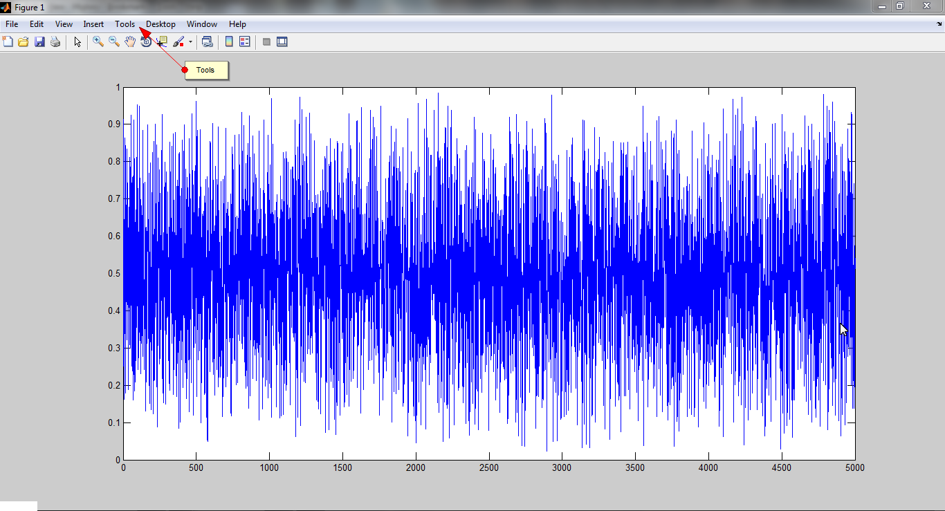
The basic fitting tool is in the Tools>Basic Fitting in the toolbar.
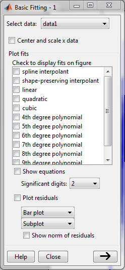
When you click the -> arrow in the above figure then you will get the complete window as shown below,
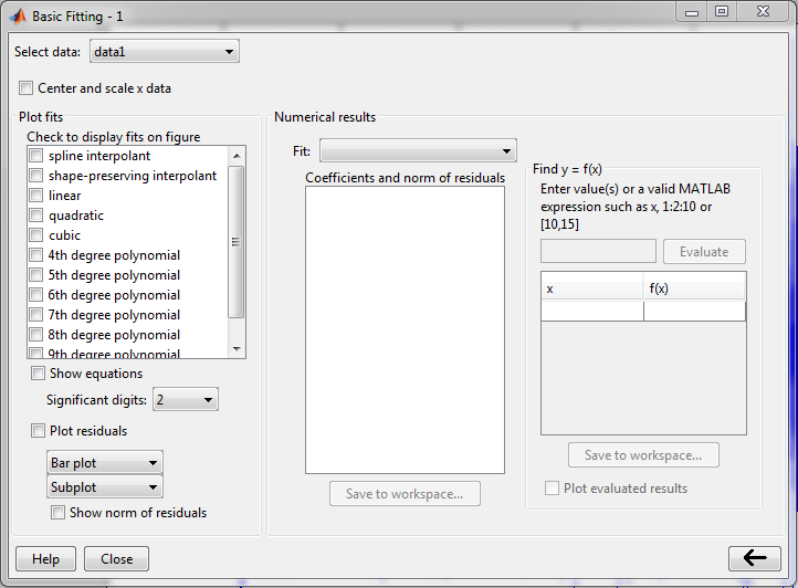
This tool window basically allows you to
The basic procedure here is now to select the interpolation algorithm that you would like to work with such as cubic or spline. Then you select the sub-option for those algorithms. Then the matlab program tries to fit the data that you have provided.
Typical when you have sets of random data, you would see the closeness of the data distribution which is done through correlation(covariance) and/or cross-correlation. The when you see any relation between any two data sets you would proceed to curve fitting.
One way to find the relationship is to find correlation between the data sets. The data set could be linearly or non-linearly relationship. Another similar statistical parameter is the covariance gives the strength of the correlation between the data sets.
This statistics can be calculated in matlab using the following 3 functions-
1. corrcoef
2. cov
3. xcorr
The first corrcoef calculates the correlation coefficient, the second cov function calculates the covariance and the third function xcorr calculates cross-correlation.
Another method of statistical analysis of random data is curve fitting. In this method, a polynomial relates input and output variables via polynomial coefficient.
A generalized polynomial equation is as follows,
y = a1 x^n + a2 x^n-1 +a3 x^n-2 + ......
The Curve fitting problem can be attacked in matlab in two ways. The first is through programming using build in functions polyfit and polyvar and others. The second approach is to use the build in Curve Fittting GUI tool.
Curve Fitting using Programming approach:
There are two matlab function which is used to analyze such polynomial equation- polyfit and polyval.
polyfit calculates the coefficients like a1, a2 .. in the above equation from data x and y. And, polyval calculates y from coefficients and x.
Curve Fitting GUI tool:
Yet another way of analyzing your data is the interactive fitting using the matlab basic fitting tool. Lets illustrate an example on how to use the basic fitting tool in matlab.
Let say you have done some experiment and collected some random data.
To opent the basic fitting tool you need to open the plot window by typing
>> plot(data)
in the matlab command prompt, where data is your random data.
Here is an example of such a plot of random data. Your plot will be different than this.

The basic fitting tool is in the Tools>Basic Fitting in the toolbar.

When you click the -> arrow in the above figure then you will get the complete window as shown below,

This tool window basically allows you to
- Select various interpolation algorithms- spline interpolant and polynomial interpolant
- Plot data in various forms
- Compute equation
- compute coefficients, residuals
- export the data
The basic procedure here is now to select the interpolation algorithm that you would like to work with such as cubic or spline. Then you select the sub-option for those algorithms. Then the matlab program tries to fit the data that you have provided.
0 comments:
Post a Comment